irdp

Follow @chazzbel

From the third quarter of 2008 to the present, the financial markets have “gone to one,” meaning that all investment options have become highly correlated. They have all gone down (with the notable exceptions of cash and government bonds). The benefit of holding uncorrelated assets is that they should not all move in lock step, so that while one goes down, hopefully another will increase. The question that this article attempts to answer is whether the long-term correlations that sales and marketing materials often quote are similar in the short term as well.

Image: Geopaul

Typically, correlation between investment assets and asset classes is calculated over extended time periods, such as 5, 10, or 15 years. But what is of greater concern to the investor is what the correlation will be next month. The use of a low 15-year correlation might obscure more recent data due to the length of time over which the correlation was calculated. Could it be, for example, that the last 12 months would show a much higher correlation between assets than the figure contained in the marketing literature?

This article looks at the near-term issues regarding correlation. Using two series of random numbers (180 observations to simulate 15 years of monthly returns) and running a short (100-trial) Monte Carlo simulation (a process that repeats the same trial), these uncorrelated random series showed significant 36-, 24-, and 12-month correlations. This suggests that investors should also consider short-term correlations between assets when attempting to diversify their portfolios. In addition, correlations should be rebalanced as often as asset allocations because investment strategies, personnel, and so forth change over time.

What is Correlation?

Most investors have the singular goal of maximizing investment return given a certain level of risk tolerance. Modern portfolio theory holds that returns are maximized in the long run when they are held in a diversified portfolio. A statistical measure of diversification is “correlation,” which is measured on a scale that runs from -1.0 to +1.0. A correlation coefficient of -1.0 or +1.0 is considered perfect correlation, knowing how one series of data moves provides perfect information on how the second series will move.

A negative correlation coefficient signifies that the two series move in opposite directions, for example, as one series increases, the other decreases. This is also known as an inverse correlation. A positive or direct correlation indicates that the series move together, as one increases, the other also increases. It is rare that one comes across perfect correlation, that is, a correlation coefficient of exactly -1.0 or +1.0.

The plus or minus sign indicates whether the relationship is direct or inverse, whereas the calculated value indicates the strength of the relationship. As the correlation coefficient moves from zero toward +1.0, there is an increasingly direct statistical relationship. Conversely, as the correlation coefficient moves from zero to -1.0, there is an increasingly inverse statistical relationship. In addition, a correlation of -0.7, then, is exactly as significant as a correlation of +0.7. A correlation coefficient of zero indicates that there is no statistical relationship between the two series of numbers, the series behave randomly with respect to one another. This is also called “non-correlation,” or, sometimes, the two series are said to be “uncorrelated.”

One important point about correlation is that it does not represent causality. For instance, in school-age children, shoe size is a great predictor of reading ability, not because shoe size has anything to do with reading, but because it is a proxy for age, older children tend to read better.

Correlation and Investing

Some investors believe that they make only three investment decisions: asset allocation, manager selection, and vehicle choice. Asset allocation is important because it is widely held that diversification is a cornerstone of investing theory. Diversification follows the logic of not putting all of your eggs in one basket. If an investor invests in a single stock, then the portfolio will do as well or as poorly as that single stock. If the investors select two stocks, they would appear to have achieved some level of diversification, but this is only at a company level. If both companies are engaged in the same industry, like Pepsi and Coca-Cola, or American Airlines and Delta, or Ford and GM, then the stock price movements that affect an industry segment will affect both stocks, that is, 100 percent of their portfolio. So, the investors might want also to diversify along company, industry, or geographical lines.

Diversification is usually quantified by correlation, that is, the degree to which the movement of one investment or asset class allows for inferences about how another investment or asset class will move. This is not indicative of causality, but simply a statistical relationship that may include causality and that can also occur simply by chance. A portfolio is not diversified if all of its holdings are correlated with one another, meaning that if one holding moves a certain way, we can predict how the other holdings will move. Brokers of commodity-based products (whether futures contracts or hard-asset ownership), infrastructure investments, and real estate funds often cite “uncorrelated with existing asset classes” as a major selling point of their products:

Issues with Non-Correlation as an Investment Strategy

Asset classes are too broad

Individual products within an asset class are not created equal; there are a wide variety of investment choices within any class. For instance, within the “hedge fund” asset class (assuming one considers hedge funds an asset class) there are over 8,000 investment choices. Treating the returns of the asset class as representative of the returns of the underlying components could be erroneous. The same is true of U.S. equities as a whole, or even when dealing with subcategories, such as Small Cap Growth, Small Cap Value, Large Cap Growth, Large Cap Value, and so forth. To be useful, non-correlation should focus on product-level asset holdings.

Not all portfolios are alike

Portfolio compositions usually differ among investors in terms of asset allocation and individual investment choices. To claim that a particular product will not be correlated with the portfolio does not give appropriate credit to the diversity of investments and the particular holdings. To be relevant, correlation should be calculated based on the returns of specific portfolio holdings, not generic asset-class returns.

Different types of non-correlation

Third, there can be different types of non-correlation. One type of non-correlation is the one people ordinarily think of when they define non-correlation, when one variable changes, the other variable will behave randomly. Another type of non-correlation operates very differently. Two series can have a low overall level of correlation even if they are 100-percent positively correlated half of the time (i.e., they have a correlation of +1.0 for half of the observations) and 100 percent negatively correlated the other half of the time (i.e., they have a correlation of -1.0 for half of the observations). In this situation, the variables clearly have some kind of relationship to one another, although the overall correlation coefficient might indicate otherwise.

Perhaps what makes correlation so interesting is that similar situations can lead to quite different results. Consider the following small series:

Observation	X	Y
1	1	9
2	2	8
3	3	7
4	4	6
5	5	5
6	4	4
7	3	3
8	1	1

The overall correlation is -.096, which is not even remotely statistically significant. But within that overall insignificant correlation are two sub-series (observations 1 to 4 and observations 5 to 8). The correlation of observations 1 to 4 is -1.0, and the correlation of observations 5 to 8 is +1.0, which are perfect correlations.

Now consider another small series:

Observation	X	Y
1	4	5
2	3	6
3	2	7
4	6	3
5	7	4
6	8	4

The correlation of observations 1 to 3 is -1.0, and the correlation of observations 4 to 6 is +1.0, as in the last series. However, the overall correlation is .72, which is on the border of statistical significance at the .10 level.

In the first case, we had an overall correlation coefficient that indicated there was absolutely no statistical relationship between the two series. However, embedded within that series were two shorter series that had extreme levels of correlation (one positive and one negative). In the second case, the observations were similarly arranged so that the first half of the series had a correlation coefficient of -1.0, and the second half of the series had a correlation coefficient of +1.0, yet the overall result was a nearly statistically significant correlation of .72.

Even when it operates as we think it does, do we want it?

If two asset classes (or individual investments) are truly uncorrelated, then when the first asset class increases, the other class may increase, decrease, or remain unchanged. There is no existing statistical relationship that allows us to infer how one class will behave based on the behavior of the other, but is this random effect desirable? We can couch the issue in the following terms: When the first asset class increases, we would like the other class to increase. However, since it is behaving randomly, there is only a one-in-three likelihood that it will do so (with the three possibilities being for it to increase, decrease, and remain unchanged). Similarly, when the first asset class decreases, we would like the other class to increase, though, again, there is a one-in-three chance this will happen. Better odds can be achieved by betting “black” at a roulette table.

The Experiment

This article examines whether uncorrelated (in the long term) series of numbers (representing investment returns) are also uncorrelated in the short term. While most investment professionals will not be surprised that uncorrelated asset classes (or investments) may have short-term correlations, the question is whether the frequency and duration of the short-term correlations are what might be expected.

This study was exploratory in nature because we could not find empirical research that quantifies the type of short-term correlation that would be considered “normal.” Since we have no basis on which to a priori establish whether the short-term series are abnormal, we will quantify and present the results and establish the literature.

We began with two series of 180 random numbers representing 15 years of monthly returns. Correlations were calculated for the last 36, 24, and 12 months of the series, since these timeframes were representative of the effect that will be introduced into the portfolio. In other words, the relevant correlation is the most recent one, not the one that was evident 15 years ago. A hundred iterations of this experiment were performed.

Exhibit 1: Frequency of observed correlations resulting from 100 trials

Each trial had 180 monthly observations (15 years). During the 100 trials, the overall correlation was .20 one time, and less than .20 the other 99 times.

The correlation for each trial was recalculated over the last 36, 24, and 12 months, and the correlations for these shorter periods are indicated:

Correlation (+/-)	0.2	0.3	0.4	0.5
Overall	1	-	-	-
Last 36 months	27	9	2	-
Last 24 months	33	18	6	2
Last 12 months	61	39	21	10

The Results

The test revealed that, overall, the two series were uncorrelated. In the 100 trials, the overall correlation of .20 was only obtained once. When we reviewed the correlations of the last 36, 24, and 12 months, some startling results were evident. In the last 36 months of each trial, the correlation was 0.2 or more 27 percent (27/100) of the time, 0.3 or more 9 percent of the time, and 0.4 or more 2 percent of the time.

For the last 24 months, a correlation of 0.2 or more occurred 33 percent of the time, a correlation of 0.3 or more resulted 18 percent of the time, a correlation of 0.4 or more was obtained 6 percent of the time, and a correlation of 0.5 or more occurred 2 percent of the time.

The last 12 months, however, may be the most relevant period because this timeframe is the most likely to impact a portfolio. A correlation of 0.2 or more occurred 61 percent of the time, a correlation of 0.3 or more was evident 39 percent of the time, a correlation of 0.4 or more occurred 21 percent of the time, and a correlation of 0.5 or more was found 10 percent of the time. An investor adding an investment and expecting it to be uncorrelated (based on 15 years worth of data) could very well be surprised at the resultant effect.

Conclusion: Do Your Short-Term Correlation Home-Work

Our findings suggest that if an investor is adding an investment to his or her portfolio with the goal of aiding diversification, he or she should parse the long-term correlation into shorter-term metrics. The nearer and the shorter the timeframe, the greater the likelihood that the investment will move from uncorrelated to correlated. As the correlation that will be added to the portfolio is more reflective of the 180th month than the first month of the series, the additional calculation of a near-term 36-, 24-, and 12-month correlation could prove useful. Perhaps there is an investment that can be added to the portfolio that, over the long term, will provide uncorrelated returns and, therefore, aid in diversification. However, if the return stream is presently correlated to the portfolio, the investor should wait a couple of periods before adding the investment, thereby mitigating the short-term effects of correlation.

Review Investments Periodically for Correlation Shifts

An additional implication from this study concerns investments that are already in the portfolio. Once an investment is added, there is usually no further attention devoted to the correlation. This study suggests, however, that the correlations of the existing investments should also be reviewed periodically. Manager changes, style drift, and so forth may mean that the original correlation that made the investment attractive is no longer accurate.

About the Author(s)

Jeffry Haber, PhD, is an associate professor of accounting at Iona College, where he teaches undergraduate and graduate classes in a variety of accounting areas. He publishes in the areas of investments, anti-money laundering and terrorist financing, earnings quality, ethics, bankruptcy prediction, and other areas of financial and managerial accounting. Haber received bachelor's and master's degrees from Syracuse University and his doctorate from Rensselaer Polytechnic Institute. He is active on a number of professional committees and is a frequent speaker at investment conferences. He is also controller of a private foundation.

Andrew Braunstein, PhD, is a professor of business economics in the Hagan School of Business at Iona College in New Rochelle, New York, where he has recently completed his 31st year of fulltime service. The majority of his research and publication activity has involved the application of econometric techniques to issues in business, economics, and education.

Risk-Return relationship in investments

The entire scenario of security analysis is built on two concepts of security: Return and risk. The risk and return constitute the framework for taking investment decision. Return from equity comprises dividend and capital appreciation. To earn return on investment, that is, to earn dividend and to get capital appreciation, investment has to be made for some period which in turn implies passage of time. Dealing with the return to be achieved requires estimated of the return on investment over the time period. Risk denotes deviation of actual return from the estimated return. This deviation of actual return from expected return may be on either side – both above and below the expected return. However, investors are more concerned with the downside risk.

The risk in holding security deviation of return deviation of dividend and capital appreciation from the expected return may arise due to internal and external forces. That part of the risk which is internal that in unique and related to the firm and industry is called ‘unsystematic risk’. That part of the risk which is external and which affects all securities and is broad in its effect is called ‘systematic risk’.

The fact that investors do not hold a single security which they consider most profitable is enough to say that they are not only interested in the maximization of return, but also minimization of risks. The unsystematic risk is eliminated through holding more diversified securities. Systematic risk is also known as non-diversifiable risk as this can not be eliminated through more securities and is also called ‘market risk’. Therefore, diversification leads to risk reduction but only to the minimum level of market risk.

The investors increase their required return as perceived uncertainty increases. The rate of return differs substantially among alternative investments, and because the required return on specific investments change over time, the factors that influence the required rate of return must be considered.

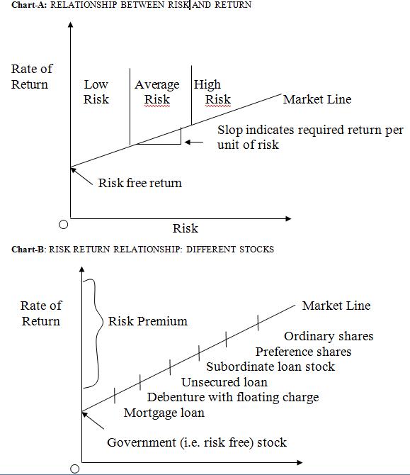
Above chart-A represent the relationship between risk and return. The slop of the market line indicates the return per unit of risk required by all investors highly risk-averse investors would have a steeper line, and Yields on apparently similar may differ. Difference in price, and therefore yield, reflect the market’s assessment of the issuing company’s standing and of the risk elements in the particular stocks. A high yield in relation to the market in general shows an above average risk element. This is shown in the Char-B

Risk and Return in Portfolio investments

Return:

The typical objective of investment is to make current income from the investment in the form of dividends and interest income. Suitable securities are those whose prices are relatively stable but still pay reasonable dividends or interest, such as blue chip companies. The investment should earn reasonable and expected return on the investments. Before the selection of investment the investor should keep in mind that certain investment like, Bank deposits, Public deposits, Debenture, Bonds, etc. will carry fixed rate of return payable periodically. On investments made in shares of companies, the periodical payments are not assured but it may ensure higher returns from fixed income securities. But these instruments carry higher risk than fixed income instruments.

Risk:

The Webster’s New Collegiate Dictionary definition of risk includes the following meanings: “……. Possibility of loss or injury ….. the degree or probability of such loss”. This conforms to the connotations put on the term by most investors. Professional often speaks of “downside risk” and “upside potential”. The idea is straightforward enough: Risk has to do with bad outcomes, potential with good ones.

In considering economic and political factors, investors commonly identify five kinds of hazards to which their investments are exposed. The following tables show components of risk:

(A)  SYSTEMATIC RISK:

1. Market Risk
2. Interest Rate Risk
3. Purchasing power Risk

(B)   UNSYSTEMATIC RISK:

1. Business Risk
2. Financial Risk

(A) Systematic Risk:

Systematic risk refers to the portion of total variability in return caused by factors affecting the prices of all securities. Economic, Political and Sociological charges are sources of systematic risk. Their effect is to cause prices of nearly all individual common stocks or security to move together in the same manner. For example; if the Economy is moving toward a recession & corporate profits shift downward, stock prices may decline across a broad front. Nearly all stocks listed on the BSE / NSE move in the same direction as the BSE / NSE index.

Systematic risk is also called non-diversified risk. If is unavoidable. In short, the variability in a securities total return in directly associated with the overall movements in the general market or Economy is called systematic risk. Systematic risk covers market risk, Interest rate risk & Purchasing power risk

1. Market Risk:

Market risk is referred to as stock / security variability due to changes in investor’s reaction towards tangible & intangible events is the chief cause affecting market risk. The first set that is the tangible events, has a ‘real basis but the intangible events are based on psychological basis.

Here, Real Events, comprising of political, social or Economic reason. Intangible Events are related to psychology of investors or say emotional intangibility of investors. The initial decline or rise in market price will create an emotional instability of investors and cause a fear of loss or create an undue confidence, relating possibility of profit. The reaction to loss will reduce selling & purchasing prices down & the reaction to gain will bring in the activity of active buying of securities.

2. Interest Rate Risk:

The price of all securities rise or fall depending on the change in interest rate, Interest rate risk is the difference between the Expected interest rates & the current market interest rate. The markets will have different interest rate fluctuations, according to market situation, supply and demand position of cash or credit. The degree of interest rate risk is related to the length of time to maturity of the security. If the maturity period is long, the market value of the security may fluctuate widely. Further, the market activity & investor perceptions change with the change in the interest rates & interest rates also depend upon the nature of instruments such as bonds, debentures, loans and maturity period, credit worthiness of the security issues.

3. Purchasing Power Risk:

Purchasing power risk is also known as inflation risk. This risks arises out of change in the prices of goods & services & technically it covers both inflation & deflation period. Purchasing power risk is more relevant in case of fixed income securities; shares are regarded as hedge against inflation. There is always a chance that the purchasing power of invested money will decline or the real return will decline due to inflation.

The behaviour of purchasing power risk can in some way be compared to interest rate risk. They have a systematic influence on the prices of both stocks & bonds. If the consumer price index in a country shows a constant increase of 4% & suddenly jump to 5% in the next. Year, the required rate of return will have to be adjusted with upward revision. Such a change in process will affect government securities, corporate bonds & common stocks.

(B) Unsystematic Risk:

The risk arises out of the uncertainty surrounding a particular firm or industry due to factors like labour Strike, Consumer preference & management policies are called Unsystematic risk. These uncertainties directly affect the financing & operating environment of the firm. Unsystematic risk is also called “Diversifiable risk”. It is avoidable. Unsystematic risk can be minimized or Eliminated through diversification of security holding. Unsystematic risk covers Business risk and Financial risk

1. Business Risk:

Business risk arises due to the uncertainty of return  which depend upon the nature of business. It relates to the variability of the business, sales, income, expenses & profits. It depends upon the market conditions for the product mix, input supplies, strength of the competitor etc. The business risk may be classified into two kind viz. internal risk and External risk.

• Internal risk is related to the operating efficiency of the firm. This is manageable by the firm. Interest Business risk loads to fall in revenue & profit of the companies.
• External risk refers to the policies of government or strategic of competitors or unforeseen situation in market. This risk may not be controlled & corrected by the firm.

2. Financial Risk:

Financial risk is associated with the way in which a company finances its activities. Generally, financial risk is related to capital structure of a firm. The presence of borrowed money or debt in capital structure creates fixed payments in the form of interest that must be sustained by the firm. The presence of these interest commitments – fixed interest payments due to debt or fixed dividend payments on preference share – causes the amount of retained earning availability for equity share dividends to be more variable than if no interest payments were required. Financial risk is avoidable risk to the extent that management has the freedom to decline to borrow or not to borrow funds. A firm with no debt financing has no financial risk. One positive point for using debt instruments is that it provides a low cost source of funds to a company at the same time providing financial leverage for the equity shareholders & as long as the earning of company are higher than cost of borrowed funds, the earning per share of equity share are increased

Using this stock investment guide may help you to acquire practical stock market experience that I paid too much to learn.

You should try to develop the ability to control personal emotions such as fear of loss or greed for a larger profit, which may affect your investment decisions.

This guide is adapted from Gerald Loeb's bestseller titled The Battle for Investment Survival. He worked as a stock broker on Wall Street for more than 40 years.

A better way to gain stock market experience

Your 'experience' fund should be small, preferably less than $10,000, even if your starting capital is in the millions. In the stock market, a $5,000 loss and a $50,000 loss teaches you similar lessons.

Part 1

Select one reputable company, preferably listed as one of the Straits Times Index component stocks Part 2

Before your purchase, write down the reason for selecting the company.

Part 3

Buy it at the time when you feel the price should go up. Subsequently, sell it at the time when you feel the price is going to drop.

One rule applies: You can buy only one stock at a time and you have to close out your position at a profit or loss in each one before switching to another stock.

When you cannot decide if you should hold or sell the stock, refer to the reason you wrote down before buying the stock. Is the reason still valid? If not, it may be time to let go.

Lessons Learned

Obviously, following this stock investment guide process is going to take time. Try it out for a few months. The method seems simple but it may not be easy to execute.

This simple exercise should show you 3 important lessons in stock investment.

1) The stock market does not care what you think,

2) your emotions, not your logic, is in control when you invest in the stock market,

3) the reason why you buy a stock in the first place should be the reason you sell when it is no longer valid.

Over the course of your buying and selling, you are likely to make some of the common mistakes made by some of my clients. How do I know? I made those mistakes too.

On paper investing and simulated investing

It sounds great in theory. Buy and sell stocks for a few months on paper or demo account and make a profit before you put any real money on the line.

The flaw in these 2 ways of gaining market experience compared to the stock investment guide above is that the psychological aspects of investing do not enter into the equation.

Fear of losing, greed for more profit, panic when market crashes, all of which may affect your investment decisions are not considered.

Don't bring that confidence over to the stock market!

If you are in the top 50 percentile of your cohort, profession, or industry, I congratulate you for achieving the success you have obtained through your hard work and commitment.

Before you climb to the top 50 percentile in your field, did you put in the time and effort to gain the necessary experience? The stock market is no different.

Just remember, the stock market is a totally different playing field from your area of specialty. Your confidence must come only from your success in the stock market.

The bottom line is, to make a killing in the stock market, figure out how not to get killed first.